R Manual

credit to Maisie Zhang, the first Stats 101 head tutor, for compiling this guide.

General

Install software

Note that you must install R before RStudio and both programs are required

R statistical package

R Studio user interface

Notes on use

Case: does differentiate between uppercase and lowercase
Variable name: consists of letters, numbers and the dot or underline characters, and starts with a letter or the dot not followed by a number
Punctuation: only English punctuation is accepted
Pound sign: # leads a comment line
Dollar sign: $ extracts elements by name from a named list and is often used as <data.frame>$<column>
Percent sign: % is not accepted as percentage and percentage needs to be expressed as fraction
Assignment operator: <- (left arrow) assigns a value to a name
- Example: x <- 2 + 3
To R, the result is a vector, even though for simple calculations the vector has only one element
Pipe operator: %>% indicates that you are passing the result of one function to the next function. Requires the tidyverse package

Install packages

R by default comes with many built-in tools however the real power of the program comes from the packages others have written to extend R.

To install a new package, there are two options:

Use the command line:

install.packages ("ggplot2")

Use the user interface:

Click Tools - Install Packages…
Type ggplot2 in Packages blank
Click Install

then, on the command line, type:

library(ggplot2)

You only need to install a package once. However, each time you restart R, you must load the library again using the library() command

Keyboard shortcuts & tips

Navigate command history: Up / Down
Clear console: Ctrl + L
Change font size: click Tools - Global Options… - Appearance - Editor Font size

Basic functions

Usually in this class we will be using dpylr package to do most calculations and data manipulation. But in some cases you may find it faster to use the base R functions.

help() : the primary interface to the help systems

example: help(mean)

A more convenient way is to type just ? and the function name. For example, help(mean) and ?mean work the same

c(): combines values into a vector or list

result <- c(1, 2)

result

[1] 1 2

mean(x, na.rm = FALSE): arithmetic mean

mean(mtcars$mpg)

[1] 20.09062

sd(x, na.rm = FALSE): sample standard deviation which uses denominator n-1

sd(mtcars$mpg)

[1] 6.026948

Note this function does NOT calculate population SD but the sample SD

summary(): for numeric variables, returns minimum, 1st quartile, median, mean, 3rd quartile, and maximum; for categorical variables, returns counts of all categories

summary(mtcars$mpg)

   Min. 1st Qu.  Median    Mean 3rd Qu.    Max. 
  10.40   15.43   19.20   20.09   22.80   33.90

Piping

The usual way to operate on data in this class is with pipes %>%; a pipe will carry over the result of one calculation to the following calculation. You can create arbitrarily long computation chains that can save you a lot of typing over using the built-in R functions.

To do some of the calculations in the following sections, you can do instead:

mean(mtcars$mpg) piped version:

mtcars %>% 
  summarize(mean = mean(mpg))

      mean
1 20.09062

We can combine the mean() and the sd() function in one command like the following:

mtcars %>% 
  summarize(mean = mean(mpg), sd = sd(mpg))

      mean       sd
1 20.09062 6.026948

Data Management

Importing datasets

All datasets in this class are in .csv format (comma separated values). To import a .csv dataset, you need to:

Click File - Import Dataset - From Text (base)…
Select the file
Make sure Heading: Yes
na.strings: if the dataset has any missing values, enter the code for missing values
Strings as factors: make sure this is ticked

In R, categorical variables are represented as factors. So be careful here as some string values that are simply ID variables should not be classified as factors. There are a number of R commands that can convert between strings and factors later if you need to clean up your dataset after importing it.

Removing datasets

rm(mtcars)

The datasets we work with in R are not very large so I don’t recommend removing any datasets from memory. Once you delete it, there is no way to recover the dataset.

Rename a dataset

mpgcars <- mtcars

Dealing with factors

R stores categorical variables as a type of variable called a factor. This is different than variables stored as simply text - R will not perform any operations in variables stored simply as text.

To convert between text and factors, you can use the following commands:

fruits <- c("apple", "pear", "banana")

# Will not work properly because the variable is a text variable
summary(fruits)

   Length     Class      Mode 
        3 character character

# The factor command will convert it to a factor so R can interpret the contents
summary(factor(fruits))

 apple banana   pear 
     1      1      1

It is not a commonly used function, but if for some reason you need to convert back to text, you can use as.character() or as.numeric()

fruits <- factor(fruits)

# Converts a factor back to text. as.numeric() does the same if the factor names are numbers
as.character(fruits)

[1] "apple"  "pear"   "banana"

Select and subset

Selecting columns

mtcars %>% 
  select(mpg)

                     mpg
Mazda RX4           21.0
Mazda RX4 Wag       21.0
Datsun 710          22.8
Hornet 4 Drive      21.4
Hornet Sportabout   18.7
Valiant             18.1
Duster 360          14.3
Merc 240D           24.4
Merc 230            22.8
Merc 280            19.2
Merc 280C           17.8
Merc 450SE          16.4
Merc 450SL          17.3
Merc 450SLC         15.2
Cadillac Fleetwood  10.4
Lincoln Continental 10.4
Chrysler Imperial   14.7
Fiat 128            32.4
Honda Civic         30.4
Toyota Corolla      33.9
Toyota Corona       21.5
Dodge Challenger    15.5
AMC Javelin         15.2
Camaro Z28          13.3
Pontiac Firebird    19.2
Fiat X1-9           27.3
Porsche 914-2       26.0
Lotus Europa        30.4
Ford Pantera L      15.8
Ferrari Dino        19.7
Maserati Bora       15.0
Volvo 142E          21.4

To select multiple columns you can do:

mtcars %>% 
  select(c(mpg, cyl))

                     mpg cyl
Mazda RX4           21.0   6
Mazda RX4 Wag       21.0   6
Datsun 710          22.8   4
Hornet 4 Drive      21.4   6
Hornet Sportabout   18.7   8
Valiant             18.1   6
Duster 360          14.3   8
Merc 240D           24.4   4
Merc 230            22.8   4
Merc 280            19.2   6
Merc 280C           17.8   6
Merc 450SE          16.4   8
Merc 450SL          17.3   8
Merc 450SLC         15.2   8
Cadillac Fleetwood  10.4   8
Lincoln Continental 10.4   8
Chrysler Imperial   14.7   8
Fiat 128            32.4   4
Honda Civic         30.4   4
Toyota Corolla      33.9   4
Toyota Corona       21.5   4
Dodge Challenger    15.5   8
AMC Javelin         15.2   8
Camaro Z28          13.3   8
Pontiac Firebird    19.2   8
Fiat X1-9           27.3   4
Porsche 914-2       26.0   4
Lotus Europa        30.4   4
Ford Pantera L      15.8   8
Ferrari Dino        19.7   6
Maserati Bora       15.0   8
Volvo 142E          21.4   4

More details on advanced select commands can be found here:

Selecting columns documentation

Selecting rows

mtcars %>% 
  filter(cyl==6)

                mpg cyl  disp  hp drat    wt  qsec vs am gear carb
Mazda RX4      21.0   6 160.0 110 3.90 2.620 16.46  0  1    4    4
Mazda RX4 Wag  21.0   6 160.0 110 3.90 2.875 17.02  0  1    4    4
Hornet 4 Drive 21.4   6 258.0 110 3.08 3.215 19.44  1  0    3    1
Valiant        18.1   6 225.0 105 2.76 3.460 20.22  1  0    3    1
Merc 280       19.2   6 167.6 123 3.92 3.440 18.30  1  0    4    4
Merc 280C      17.8   6 167.6 123 3.92 3.440 18.90  1  0    4    4
Ferrari Dino   19.7   6 145.0 175 3.62 2.770 15.50  0  1    5    6

As with the column example, multiple criteria can be used:

mtcars %>% 
  filter(cyl==6 & hp==110)

                mpg cyl disp  hp drat    wt  qsec vs am gear carb
Mazda RX4      21.0   6  160 110 3.90 2.620 16.46  0  1    4    4
Mazda RX4 Wag  21.0   6  160 110 3.90 2.875 17.02  0  1    4    4
Hornet 4 Drive 21.4   6  258 110 3.08 3.215 19.44  1  0    3    1

More details on advanced filter commands can be found here:

Filtering rows documentation

Recoding variables

The main dplyr verb for recoding a variable is mutate. With mutate, you can either simply rescale a variable or do more complex transformations, such as the following:

# Weight is defined as 1000s of pounds; a ton is 2000 pounds
mtcars <- mtcars %>% 
  mutate(tons = (wt / 2000) * 1000)

A more complex transformation using the helper function case_when:

# Note we need to convert the strings to a factor after the case_when call
mtcars <- mtcars %>% 
  mutate(cartype = case_when(
    tons < 1 ~ "light",
    tons >= 1 & tons < 2 ~ "medium",
    tons > 2 ~ "heavy"
  )) %>% 
  mutate(cartype = factor(cartype))

More details on advanced mutate commands can be found here:

Mutate documentation

More details on advanced case_when commands can be found here:

Case when documentation

Missing values

Many datasets have missing values (for a variety of reasons). It is always important to check if your dataset has any missing values (in R, these are stored by default as NA).

To check the total number of missing values, we can use the following:

mtcars.missing <- mtcars

# Make the first observation missing
mtcars.missing[1,1] <- NA

colSums(is.na (mtcars.missing))

    mpg     cyl    disp      hp    drat      wt    qsec      vs      am    gear 
      1       0       0       0       0       0       0       0       0       0 
   carb    tons cartype 
      0       0       0

Most functions in R have a flag to remove missing values. If there is a missing value, the function will return an error if the flag is not set.

mean(mtcars.missing$mpg)

[1] NA

mean(mtcars.missing$mpg, na.rm=TRUE)

[1] 20.06129

Sometimes cases with missing values suggest that certain types of observations are not stored properly. It is always important to check if there are any patterns in the observations with missing values before removal.

Helpful summary functions

Summarizing data

The simpliest way to summarize data is the summary() command.

summary(mtcars$mpg)

   Min. 1st Qu.  Median    Mean 3rd Qu.    Max. 
  10.40   15.43   19.20   20.09   22.80   33.90

To develop more complex summary statistics, you can use longer piped structures from dplyr as follows:

mtcars %>%
  group_by(cyl) %>%
  summarise(mean = mean(wt), n = n())

# A tibble: 3 × 3
    cyl  mean     n
  <dbl> <dbl> <int>
1     4  2.29    11
2     6  3.12     7
3     8  4.00    14

To view more samples of the summarize() function, see here:

Summarize documetation

Finding normal distribution & quantile information

If you want to find out details of the normal distribution, there are a suite of function in R that can report the quantile of a specific number of standard deviations from the center of a normal distribution or the reverse.

# What is the amount of area under the normal curve cumulative up to +2 sd from the mean 
pnorm(2, mean=0, sd=1)

[1] 0.9772499

# At how many standard deviations away from the mean is 97.5% of the area under the normal curve
qnorm(0.975, mean=0, sd=1)

[1] 1.959964

If you have an arbitrary distribution (that may not necessarily be normally distributed), you can find a quantile for a given percentage of area under the curve with the quantile() function.

# generate a uniform distribution
dist<-runif(1000, min=0, max=1)

# theoretically, the quantile should match the probability for a uniform distribution
quantile(dist, probs=0.5)

      50% 
0.4814989

Tables & Plots

Frequency table and contingency table

Creating a frequency table is quite easy in R.

table(mtcars$cyl, mtcars$gear)

addmargins(table(mtcars$cyl, mtcars$gear))

     
       3  4  5 Sum
  4    1  8  2  11
  6    2  4  1   7
  8   12  0  2  14
  Sum 15 12  5  32

So is making a contingency table.

prop.table(table(mtcars$cyl, mtcars$gear))

   
          3       4       5
  4 0.03125 0.25000 0.06250
  6 0.06250 0.12500 0.03125
  8 0.37500 0.00000 0.06250

addmargins(prop.table(table(mtcars$cyl, mtcars$gear)))

     
            3       4       5     Sum
  4   0.03125 0.25000 0.06250 0.34375
  6   0.06250 0.12500 0.03125 0.21875
  8   0.37500 0.00000 0.06250 0.43750
  Sum 0.46875 0.37500 0.15625 1.00000

Changing the method of calculating the margins can be done with the margin option.

prop.table(table(mtcars$cyl, mtcars$gear), margin=1)

   
             3          4          5
  4 0.09090909 0.72727273 0.18181818
  6 0.28571429 0.57142857 0.14285714
  8 0.85714286 0.00000000 0.14285714

prop.table(table(mtcars$cyl, mtcars$gear), margin=2)

   
             3          4          5
  4 0.06666667 0.66666667 0.40000000
  6 0.13333333 0.33333333 0.20000000
  8 0.80000000 0.00000000 0.40000000

Histogram

Histograms are quite easy using ggplot.

ggplot(mtcars, aes(x=wt)) +
  geom_histogram()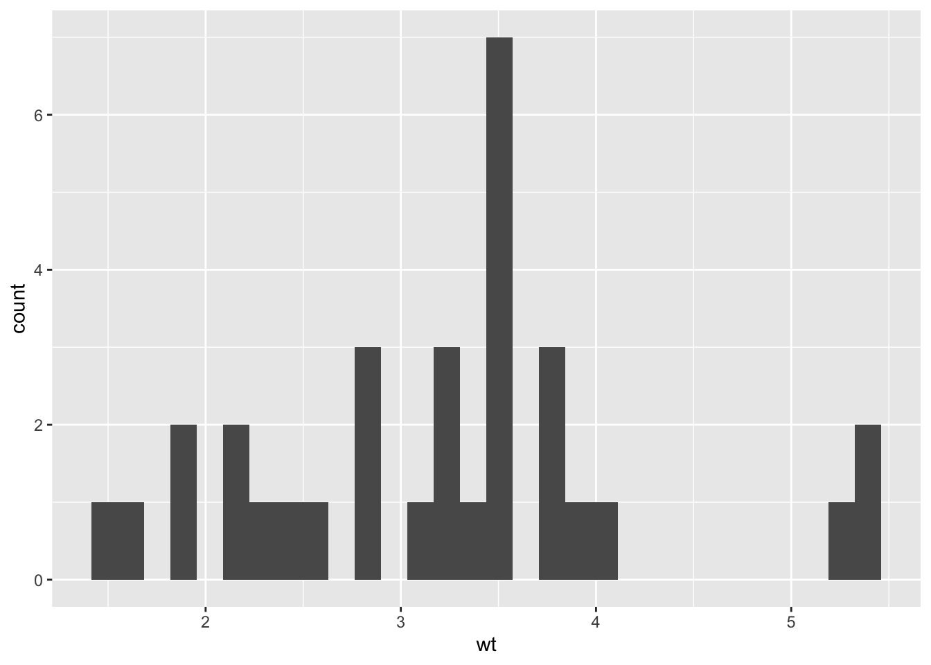

Details on how to modify the graphical parameters of geom_histogram() can be found here:

Histogram documetation

Remember, histograms should only be use for quantitative data. Even if a categorical variable is numeric (cylinders, for example), you should represent that variable with a bar chart.

Boxplot

Boxplots are useful if you want to compare the distribution of a variable across several different categories. For example, boxplots are a good way to compare the distribution of car weight by number of cylinders in a car.

ggplot(mtcars, aes(x=factor(cyl), y=wt)) +
  geom_boxplot()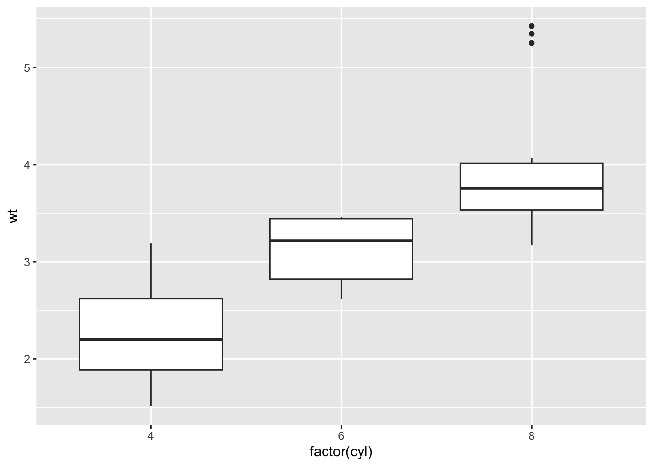

The grouping variable x must be categorical in the box plot call

Details on how to modify the graphical parameters of geom_boxplot() can be found here:

Boxplot documetation

Bar chart

Bar charts are the best way to display the distribution of categorical variables. Since we generally don’t assign importance to the order or distance between categories, we can only simply show the count of each category independently.

ggplot(mtcars, aes(x=factor(cyl))) +
  geom_bar()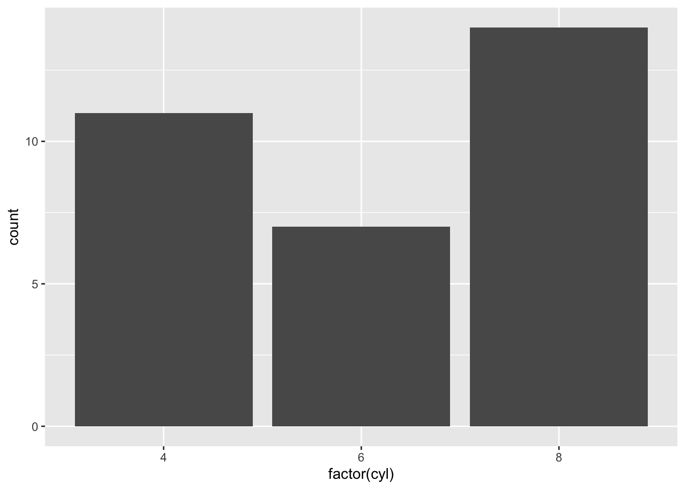

Details on how to modify the graphical parameters of geom_bar() can be found here:

Bar chart documetation

QQ Plot in ggplot

QQ plots are useful to determine if a distribution is normal shaped. While we won’t discuss it in this class, it may be helpful for certain projects you work on. Similar to other singe variable ggplots, you can create one as follows:

ggplot(mtcars, aes(sample=wt)) +
  geom_qq() +
  geom_qq_line()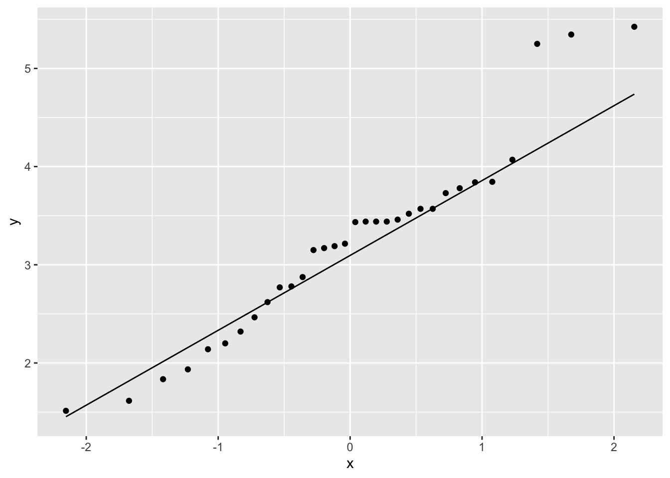

Information on how to interpret these plots can be found in Chapter 5 of the textbok.

Details on how to modify the graphical parameters of geom_qq() can be found here:

QQ plot documetation

Scatterplot in ggplot

Scatterplots are the most common way to display a two-variable relationship and are one of the most common graphical displays.

ggplot(mtcars, aes(x=wt, y=mpg)) +
  geom_point()

Remember that your response variable should always be on the y axis on a scatterplot

It is relatively common to add a line of best fit into a scatterplot to summarize the relationship between the two variables. You can do so by using the geom_smooth() function.

ggplot(mtcars, aes(x=wt, y=mpg)) +
  geom_point() +
  geom_smooth(method=lm, se=FALSE)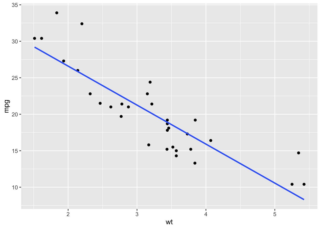

There are a number of different options for how to choose a best fit line, remember to select the one that you think best represents the relationship between the two variables.

Details on how to modify the graphical parameters of geom_point() and geom_smooth() can be found here:

Scatterplot documetation

Smoother documetation

Correlation in ggcorrplot

One helpful graphical display to quickly summarize the relationship between many variables is a correlation plot. It displays the correlation between the variables you specify in your dataset. First, you need to work out which variables you want to include in the correlation matrix.

mtcars.subset <- mtcars %>% 
  select(c(mpg, cyl, wt, disp))

# use = complete.obs here in case of missing values
mtcars.cor <- cor(mtcars.subset, use="complete.obs")

mtcars.cor

            mpg        cyl         wt       disp
mpg   1.0000000 -0.8521620 -0.8676594 -0.8475514
cyl  -0.8521620  1.0000000  0.7824958  0.9020329
wt   -0.8676594  0.7824958  1.0000000  0.8879799
disp -0.8475514  0.9020329  0.8879799  1.0000000

Then simply use the ggcorrplot() function.

ggcorrplot(mtcars.cor)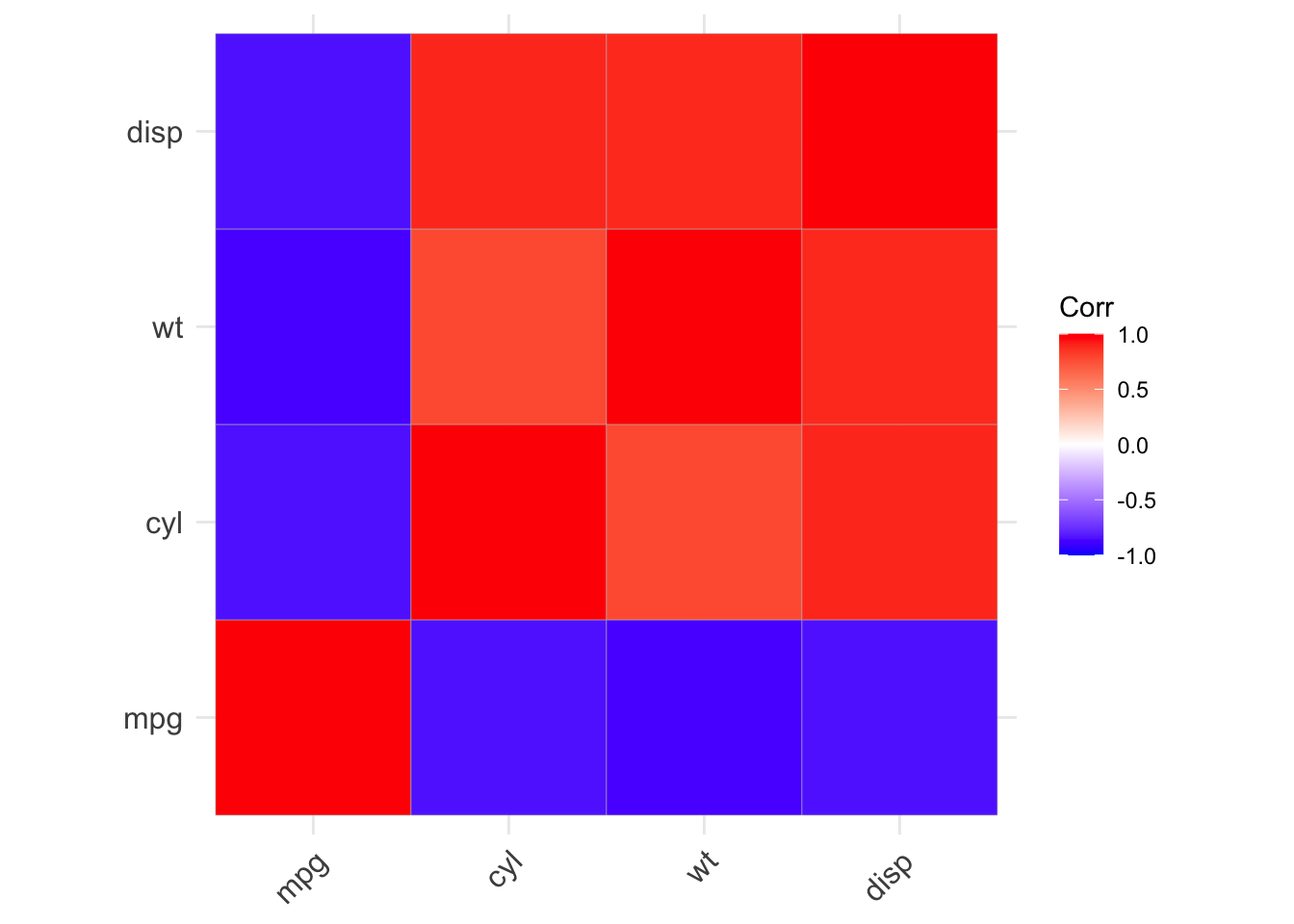

Details on how to modify the graphical parameters of ggcorrplot() can be found here:

ggcorrplot documetation

Adding features to ggplots

You can modify ggplots to add many different features. Below is a short list of basic things you can add but this is not by far a complete list.

Change the colors and lines

ggplot (mtcars, aes(x = wt)) + 
  geom_histogram(fill = "#FF6666", alpha = 0.8, color = "black", linetype = "dashed", size = 1)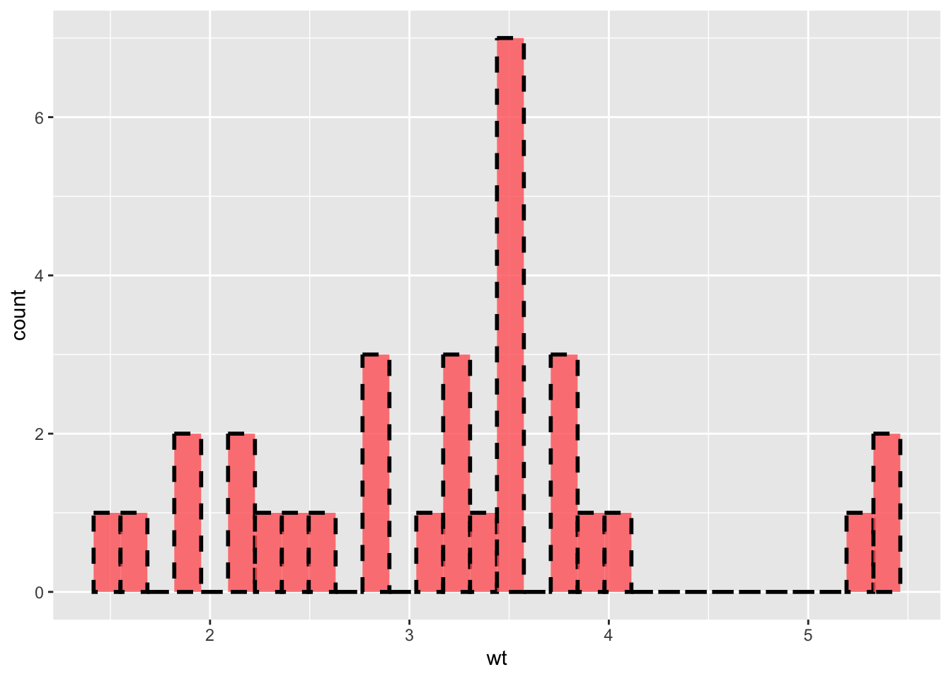

Add labels and title

ggplot(mtcars, aes (x = wt)) + 
  geom_histogram() +
  xlab("Weight") +
  ylab ("Count") + 
  ggtitle("Weight of Cars in the MPG Dataset")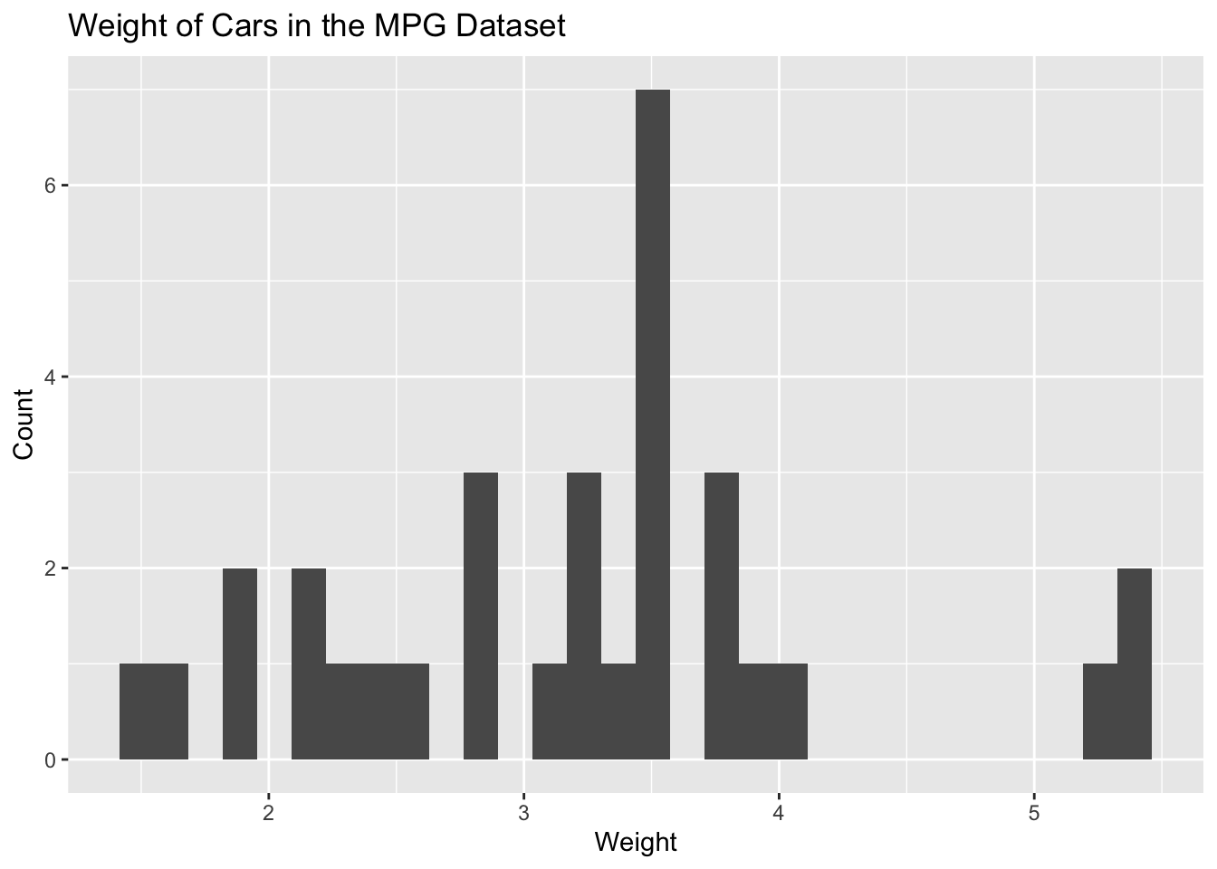

Add lines to the graph

ggplot(mtcars, aes(x = wt)) + 
  geom_histogram () + 
  geom_vline(aes(xintercept = mean(wt))) + 
  geom_hline(aes(yintercept = 3))

Arrange multiple ggplot plots

Often it can be helpful to combine many plots of the same time (histograms, for example) into one larger plot. To do this, you will need to install the gridExtra package.

library(gridExtra)

p1 <- ggplot(mtcars, aes(x = wt)) + 
  geom_histogram ()

p2 <- ggplot(mtcars, aes(x = hp)) + 
  geom_histogram ()

grid.arrange(p1, p2)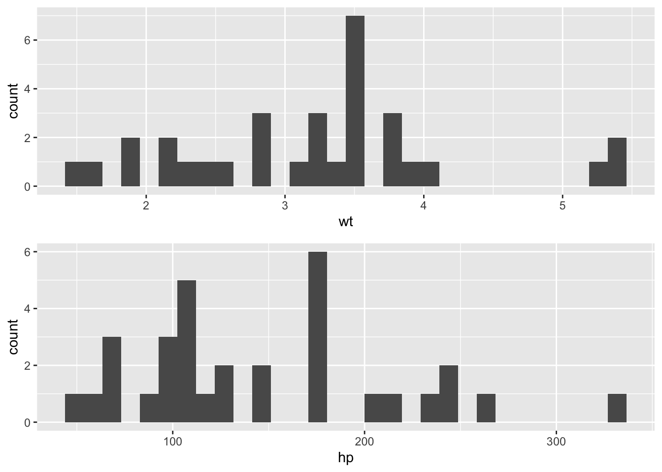

Details on how to modify the graphical parameters of grid.arrange() can be found here:

gridExtra documentation

Multiple variable analysis

Correlation

The default dplyr method of calculating a correlation can only do a two variable comparison.

mtcars %>% 
  summarize(cor(wt, mpg))

  cor(wt, mpg)
1   -0.8676594

To calculate the correlation between many variables, we can use the advanced package corrr as follows:

library(corrr)

mtcars %>% 
  select(c(mpg, disp, wt)) %>% 
  correlate()

# A tibble: 3 × 4
  term     mpg   disp     wt
  <chr>  <dbl>  <dbl>  <dbl>
1 mpg   NA     -0.848 -0.868
2 disp  -0.848 NA      0.888
3 wt    -0.868  0.888 NA

The corrr package has many advanced features and graphical capabilities if you need to calculate something more specific than the correlation matrix of the dataset.

Details on corr() can be found here:

corrr documentation

Simple regression

Calculating the regression coefficients

The standard way to calculate a regression is as follows, with the response variable on the left and the predictor variable on the right:

fit <- lm(data=mtcars, mpg ~ wt)

summary(fit)


Call:
lm(formula = mpg ~ wt, data = mtcars)

Residuals:
    Min      1Q  Median      3Q     Max 
-4.5432 -2.3647 -0.1252  1.4096  6.8727 

Coefficients:
            Estimate Std. Error t value Pr(>|t|)    
(Intercept)  37.2851     1.8776  19.858  < 2e-16 ***
wt           -5.3445     0.5591  -9.559 1.29e-10 ***
---
Signif. codes:  0 '***' 0.001 '**' 0.01 '*' 0.05 '.' 0.1 ' ' 1

Residual standard error: 3.046 on 30 degrees of freedom
Multiple R-squared:  0.7528,    Adjusted R-squared:  0.7446 
F-statistic: 91.38 on 1 and 30 DF,  p-value: 1.294e-10

There is not a particularly elegant means of calculating regressions using the tidy package, however, it is often useful, particularly when conducting many regressions, to use the broom package to return the regression results in a data frame.

library(broom)

tidy(fit)

# A tibble: 2 × 5
  term        estimate std.error statistic  p.value
  <chr>          <dbl>     <dbl>     <dbl>    <dbl>
1 (Intercept)    37.3      1.88      19.9  8.24e-19
2 wt             -5.34     0.559     -9.56 1.29e-10

For more details on tidy(), you can go here:

tidy documentation

Graphing the residuals

To graph the residuals, we can use the augment() function from the broom package to add in the residuals into the results.

aug.fit <- augment(fit)

aug.fit

# A tibble: 32 × 9
   .rownames           mpg    wt .fitted .resid   .hat .sigma .cooksd .std.resid
   <chr>             <dbl> <dbl>   <dbl>  <dbl>  <dbl>  <dbl>   <dbl>      <dbl>
 1 Mazda RX4          21    2.62    23.3 -2.28  0.0433   3.07 1.33e-2    -0.766 
 2 Mazda RX4 Wag      21    2.88    21.9 -0.920 0.0352   3.09 1.72e-3    -0.307 
 3 Datsun 710         22.8  2.32    24.9 -2.09  0.0584   3.07 1.54e-2    -0.706 
 4 Hornet 4 Drive     21.4  3.22    20.1  1.30  0.0313   3.09 3.02e-3     0.433 
 5 Hornet Sportabout  18.7  3.44    18.9 -0.200 0.0329   3.10 7.60e-5    -0.0668
 6 Valiant            18.1  3.46    18.8 -0.693 0.0332   3.10 9.21e-4    -0.231 
 7 Duster 360         14.3  3.57    18.2 -3.91  0.0354   3.01 3.13e-2    -1.31  
 8 Merc 240D          24.4  3.19    20.2  4.16  0.0313   3.00 3.11e-2     1.39  
 9 Merc 230           22.8  3.15    20.5  2.35  0.0314   3.07 9.96e-3     0.784 
10 Merc 280           19.2  3.44    18.9  0.300 0.0329   3.10 1.71e-4     0.100 
# ℹ 22 more rows

And then we can graph the residuals as follows:

ggplot(aug.fit, aes(x=.fitted, y=.resid)) +
  geom_point()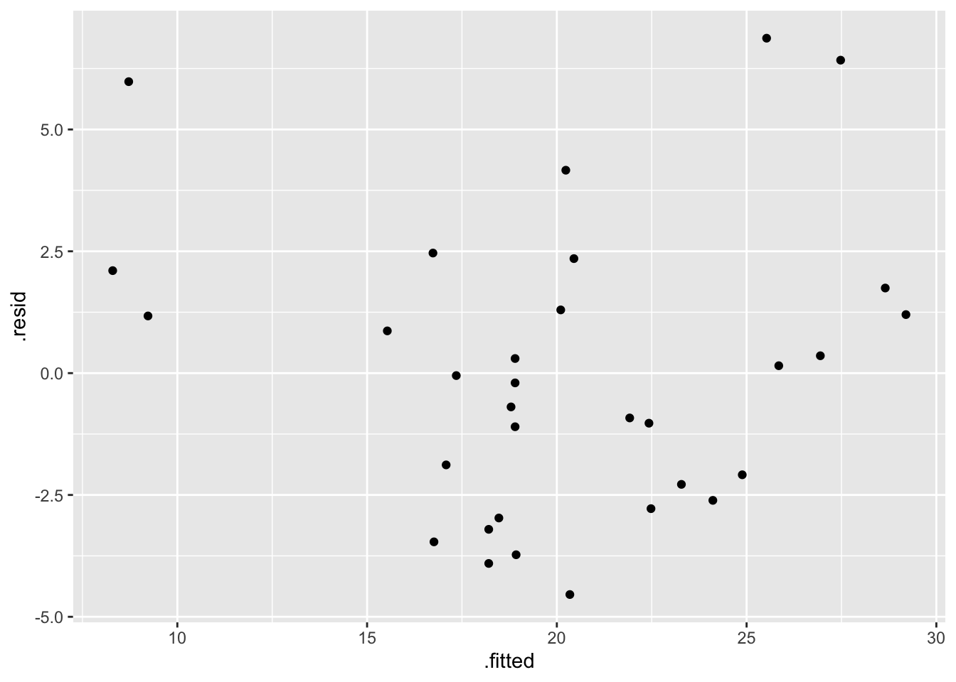

ggplot(aug.fit, aes(x=.resid)) +
  geom_histogram()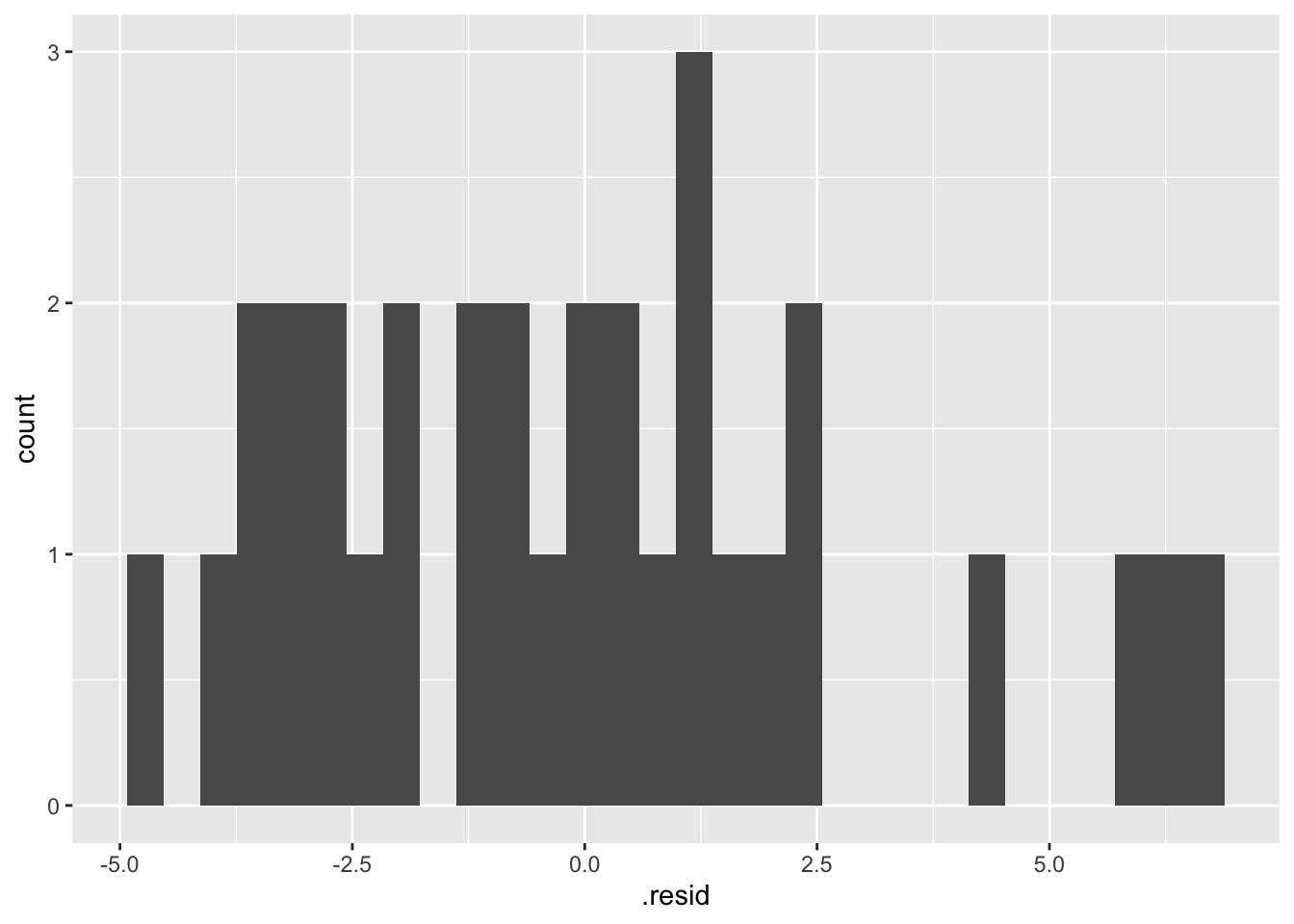

Multiple regression

Multiple regression works similarly to two variable regressions. You can easily construct advanced models (including categorical predictors and interaction terms) using the lm() command:

# Three variable regression
mod1 <- lm(data=mtcars, mpg~disp+wt)
tidy(mod1)

# A tibble: 3 × 5
  term        estimate std.error statistic  p.value
  <chr>          <dbl>     <dbl>     <dbl>    <dbl>
1 (Intercept)  35.0      2.16        16.2  4.91e-16
2 disp         -0.0177   0.00919     -1.93 6.36e- 2
3 wt           -3.35     1.16        -2.88 7.43e- 3

# Model with a categorical predictor
mod2 <- lm(data=mtcars, mpg~wt+factor(cyl))
tidy(mod2)

# A tibble: 4 × 5
  term         estimate std.error statistic  p.value
  <chr>           <dbl>     <dbl>     <dbl>    <dbl>
1 (Intercept)     34.0      1.89      18.0  6.26e-17
2 wt              -3.21     0.754     -4.25 2.13e- 4
3 factor(cyl)6    -4.26     1.39      -3.07 4.72e- 3
4 factor(cyl)8    -6.07     1.65      -3.67 9.99e- 4

# Model with an interaction term
mod3 <- lm(data=mtcars, mpg~wt+factor(cyl)+factor(cyl)*wt)
tidy(mod3)

# A tibble: 6 × 5
  term            estimate std.error statistic  p.value
  <chr>              <dbl>     <dbl>     <dbl>    <dbl>
1 (Intercept)        39.6       3.19    12.4   2.06e-12
2 wt                 -5.65      1.36    -4.15  3.13e- 4
3 factor(cyl)6      -11.2       9.36    -1.19  2.44e- 1
4 factor(cyl)8      -15.7       4.84    -3.24  3.22e- 3
5 wt:factor(cyl)6     2.87      3.12     0.920 3.66e- 1
6 wt:factor(cyl)8     3.45      1.63     2.12  4.34e- 2

Graphing partial residual plots

Partial residual plots help graphically display the relationship between a single predictor variable and the response variable after controlling for, or partialling out, the effect of all other predictor variables. If your regression specification meets all of the conditions for linear regression, this plot will illustrate the independent impact of the predictor variable on the response variable.

There are a few packages that can generate these plots, car being perhaps the best supported.

library(car)

crPlots(mod1, terms = ~ ., layout = NULL)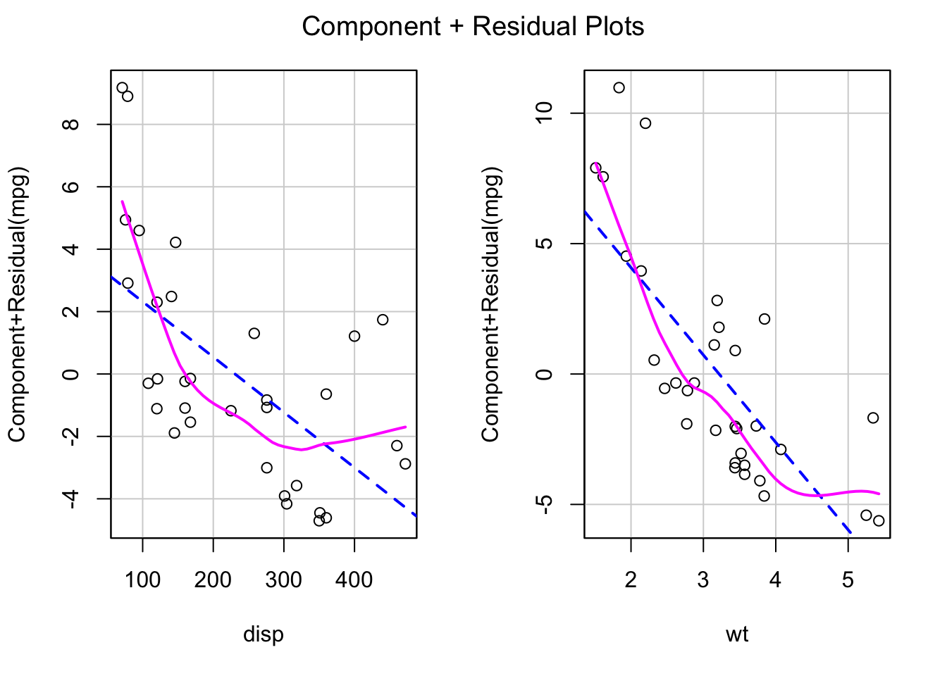

You can interpret these graphs as displaying the change in MPG from the mean (listed on the y axis) as displ or wt changes over its range. These are a type of marginal plots - it show the marginal impact of the predictor variable on the response variable after controlling for the impact of all other variables.

Note that in the crPlot() call, the terms function is a one-sided formula that specifies a subset of the predictor variables for which you would like to generate plots. One component-plus-residual plot is drawn for each regressor. The default ~ . is to plot all numeric regressors. You can modify this term to subtract terms with the specification terms = ~ . - X3, which would plot against all regressors except for X3, while terms = ~ log(X4) would give the plot for the predictor X4 that is represented in the model by log(X4). If this argument is a quoted name of one of the predictors, the component-plus-residual plot is drawn for that predictor only.

For the layout option, if set to a value like c(1, 1) or c(4, 3), the layout of the graph will have this many rows and columns. If not set, the program will select an appropriate layout. If the number of graphs exceed nine, you must select the layout yourself, or you will get a maximum of nine per page.

For more details on crPlots(), you can go here:

crPlots documentation

Confidence intervals

Confidence interval for proportion

To calculate the confidence interval of a proportion, there are often several steps involved. First you will need to possibly recode the variable and select the cases of interest, then obtain two properties of the sample (sample proportion, sample standard deviation) and find the appropriate $z$ score ($z^*$) needed for your confidence interval.

Remember to check the necessary conditions first!

Recode variable

It is easiet to work with the variable if successes are marked as 1 and failures maked as 0 in the dataset. You may want to recode your variable to make your calculations easier (see Recoding Variables)

mtcars <- mtcars %>% 
  mutate(heavy = case_when(
    tons < 1.5 ~ 0,
    tons >= 1.5 ~ 1 
  ))

Sample proportion and standard deviation

First we need to find the key features of our sample.

heavy.sum.data <- mtcars %>% 
  summarize(prop = mean(heavy),
            len = length(heavy)) %>% 
  mutate(sd = sqrt(prop*(1-prop)/len))

heavy.sum.data

   prop len         sd
1 0.625  32 0.08558165

Remember, the formula for sample sd is $\sigma(\hat{p})=\sqrt{\frac{pq}{n}}$

Confidence interval

First we need to calculate the margin of error (MOE). In the below example we are interested in a 95% confidence interval. qnorm(0.975) finds the appropriate value of $z^*$ .

heavy.sum.data <- heavy.sum.data %>% 
  mutate(moe = sd * qnorm(0.975))

Finally, we both subtract and add the MOE to the sample proportion to find the confidence interval.

heavy.sum.data$prop + c(-heavy.sum.data$moe, heavy.sum.data$moe)

[1] 0.457263 0.792737

Confidence interval for mean

The R procedure for mean confidence intervals is very similar to proportions, differing only in the method of calculating the standard deviation, which must be done using the sd() function.

Remember to check the necessary conditions first!

mpg.sum.data <- mtcars %>% 
  summarize(mean = mean(mpg),
            len = length(mpg),
            sd = sd(mpg)) %>% 
  mutate(moe = sd * qnorm(0.975),
         lower.bound = mean - moe,
         upper.bound = mean + moe)

c(mpg.sum.data$lower.bound, mpg.sum.data$upper.bound)

[1]  8.278024 31.903226

Hypothesis tests

Hypothesis test for proportion

If we are interested in testing whether there are more heavy cars with 6 cylinders compared to the overall proportion of heavy cars, the R code for such a test is relatively straightforward.

Remember to check the necessary conditions first!

First, identify the hypotheses and calculate the sample information.

$H_0: 6cyl.heavy.prop = 0.625$

$H_a: 6cyl.heavy.prop \neq 0.625$

mean.heavy <- mean(mtcars$heavy)

hyp.test.prop <- mtcars %>% 
  filter(cyl==6) %>% 
  summarize(prop = mean(heavy),
            len = length(heavy),
            sd = sqrt(mean.heavy*(1-mean.heavy)/len))

Note that the sd is calculated as if the null hypothesis were true; we use the population mean to calculate here.

Next, calculate the $z$ distance between the sample and the population mean.

z.score <- (hyp.test.prop$prop - mean.heavy)/hyp.test.prop$sd

z.score

[1] -0.29277

Finally, we find the $p$ value for that difference and compare it to our $\alpha$ value.

# Note that our test was specified as two sided, therefore we need to multiply by 2
p.value <- (pnorm(-abs(z.score)))*2

p.value

[1] 0.7696979

There is a 77% chance that one would observe a difference that large or larger from the sample mean by simple sample variation. In other words, we fail to reject the null hypothesis if our $\alpha$ is 5%.

Hypothesis test for mean

Hypothesis test for the means are very similar, though in this case we use the sample sd to estimate the population sd.

Remember to check the necessary conditions first!

mean.mpg <- mean(mtcars$mpg)

hyp.test.mean <- mtcars %>% 
  filter(cyl==6) %>% 
  summarize(mean = mean(mpg),
            len = length(mpg),
            sd = sd(mpg)/sqrt(len))

Instead of calculating a $z$ score, because of the need to correct for small sample bias, we must use the $t$ distribution.

t.score <- (hyp.test.mean$mean - mean.mpg) / hyp.test.mean$sd
df.test <- hyp.test.mean$len - 1

p.value <- pt(-abs(t.score), df=df.test)*2

p.value

[1] 0.5500829

There is a 55% chance that one would observe a difference that large or larger from the sample mean by simple sample variation. In other words, we fail to reject the null hypothesis if our $\alpha$ is 5%.

Inference for Difference between Two Samples

The R code for $t$ tests is very similar to the code for hypothesis testing.

fourcyl <- mtcars %>% 
  filter(cyl==4) %>% 
  summarize(mean=mean(mpg),
            len=length(mpg),
            sd=sd(mpg))

eightcyl <- mtcars %>% 
  filter(cyl==8) %>% 
  summarize(mean=mean(mpg),
            len=length(mpg),
            sd=sd(mpg))

diff.sd <- sqrt(fourcyl$sd ^ 2 / fourcyl$len + eightcyl$sd ^ 2 / eightcyl$len)
diff.mpg.t  <- (fourcyl$mean - eightcyl$mean) / diff.sd

# Note that the df here is just an approximation; the textbook provides the correct formula.
# The rule of thumb method from the the textbook recommends using the lowest df of the two samples
# minus one.
diff.mpg.p  <- 2 * pt(-abs(diff.mpg.t), df = min(c(fourcyl$len, eightcyl$len))-1)

diff.mpg.p

[1] 1.847002e-05

In other words, the odds that, assuming the two samples have the same sample mean, the odds that we would see a difference between the two sample means this large or larger is effectively zero, therefore we can reject the null hypothesis.

R does have a built-in method to do this calculation but you should understand how to achieve the same result by direct calcuation.

fourcyl.data <- mtcars %>% 
  filter(cyl==4) %>% 
  select(mpg)

eightcyl.data <- mtcars %>% 
  filter(cyl==8) %>% 
  select(mpg)

t.test(fourcyl.data$mpg, eightcyl.data, alternative = "two.sided" , mu = 0, var.equal = FALSE, conf.level = 0.95)


    Welch Two Sample t-test

data:  fourcyl.data$mpg and eightcyl.data
t = 7.5967, df = 14.967, p-value = 1.641e-06
alternative hypothesis: true difference in means is not equal to 0
95 percent confidence interval:
  8.318518 14.808755
sample estimates:
mean of x mean of y 
 26.66364  15.10000

Due to the first method using a rule of thumb method for calculating the degrees of freedom, the result is slightly different but very close to the R function result.