Lecture 3.2 - Confidence Intervals - Means

Confidence intervals - means

• The central limit theorem
• A confidence interval for the mean
• Interpreting confidence intervals
• Picking our interval up by our bootstraps
• Thoughts about confidence intervals

House price revisited

• Prices in King County Houses:
  • 21937 houses
  • Highly right skewed
  • Can define this as the entire population
  • Prices are quantitative

House price graph

Distribution

• Distribution:

  • Min: 75000
  • Q1: 685000
  • Med: 906000
  • Q3: 1355000
  • Max: 23000000
  • Mean: 1152092
  • SD: 835505

• Highly right skewed

• SD almost as large as the median

• If a distribution looks like this, what do you think the sampling distribution will look like when n=25? How about when n=200?

The central limit theorem

• The Central Limit Theorem
  • The sampling distribution of any mean becomes nearly Normal as the sample size grows.
• Requirements
  • Observations independent
  • Randomly collected sample
• The sampling distribution of the means is close to Normal if either:
  • Large sample size
  • Population close to Normal

Samples = 100, $n$ = 200

Samples = 1000, $n$ = 200

Samples = 100000, $n$ = 200

Sampling distribution shape

• As number of samples taken goes to infinity, shape of the sampling distribution becomes more clearly normally shaped

• Doesn’t matter the shape of the underlying distribution except for a very few exceptions

• How about holding samples fixed and changing $n$ in our sample of a skewed distribution?

$n$ = 10

$n$ = 25

$n$ = 50

$n$ = 100

Central limit theorem formally

• When a random sample is drawn from any population with mean $\mu$ and standard deviation $\sigma$, its sample mean, $\bar{y}$, has a sampling distribution with the same mean but whose standard deviation is $\frac{\sigma}{\sqrt{n}}$ and we write $\sigma(\bar{y})=SD(\bar{y})=\frac{\sigma}{\sqrt{n}}$

• No matter what population the random sample comes from, the shape of the sampling distribution is approximately Normal as long as the sample size is large enough.

• The larger the sample used, the more closely the Normal approximates the sampling distribution for the mean.

• Practically, $n$ does not have to be very large for this to work in most cases

Practical issue with finding the sampling distribution sd

• We almost never know $\sigma$

• Natural thing is to use $\hat{sd_{sample}}$

• With this, we can estimate the sampling distribution SD with SE:

  • $SE(\bar{y})=\frac{s}{\sqrt{n}}$

• This formula works well for large samples, not so much for small

  • Problem: too much variation in the sample SD from sample to sample

• For smaller $n$, need to turn to Gosset and a new family of models depending on sample size

A confidence interval for the mean

Gosset the brewer

Guiness

Gosset

Gosset

What Gosset discovered

• At Guinness, Gosset experimented with beer.

• The Normal Model was not right, especially for small samples.

• Still bell shaped, but details differed, depending on $n$

• Came up with the “Student’s $t$ Distribution” as the correct model

A practical sampling distribution model

• When certain assumptions and conditions are met, the standardized sample mean is:

$t=\frac{\bar{y}-\mu}{SE(\bar{y})}$

• The t score indicates that the result should be interpreted by a Student’s $t$ model with $n-1$ degrees of freedom

• We can estimate the standard deviation of the sampling distribution by:

$SE(\bar{y}) = \frac{s}{\sqrt{n}}$

Degrees of freedom

• For every sample size $n$, there is a different Student’s $t$ distribution

• Degrees of freedom: $df=n-1$

• Similar to the $n-1$ calculation for sample standard deviation

• Reason for this is a bit complicated, at this point can just remember to specify $t$ distribution with $n-1$

Student’s $t$

Student’s t

One sample $t$ interval for the mean

• When the assumptions are met, the confidence interval for the mean is:

$\bar{y} \pm t_{n-1}\times SE(\bar{y})$

• The critical value, $t^*_{n-1}$, depends on the confidence interval, $C$, and the degrees of freedom $n-1$

Example: A one sample $t$ interval for the mean

• Price from one sample in King County

Average house price

• $\bar{y}\pm t^*_{19} \times SE(\bar{y})$

• $1118400\pm 2.09 \times SE(\frac{789011}{\sqrt{(20)}})$

• $1118400\pm 2.09 \times 176428.33$

• $[739538 - 1497262]$

What is the right way to talk about this confidence interval?

Thoughts about $z$ and $t$

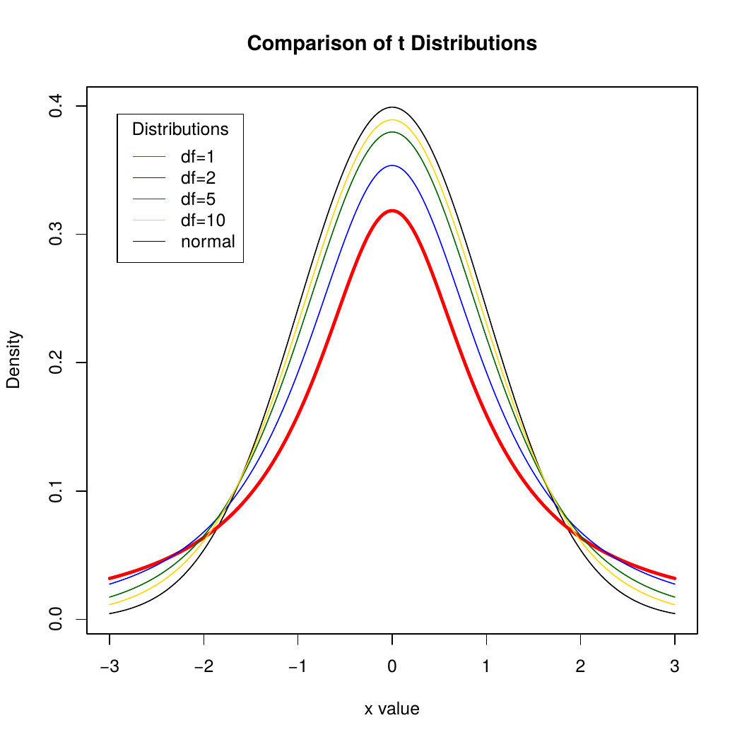
• The Student’s t distribution:

  • Is unimodal.
  • Is symmetric about its mean.
  • Bell-shaped

• Samller values of $df$ have longer tails and larger standard deviation than the Normal.

• As $df$ increase, look more and more like Normal.

• Is needed because we are using s as an estimate for $\sigma$

• If you happen to know $\sigma$, which almost never happens, use the Normal model and not Student’s $t$

• As $n$ becomes larger, still safe to use the $t$ distribution because it basically turns into the normal distribution

Assumptions and conditions

• Independence Assumption
  • Data values should be mutually independent
  • Example: weighing yourself every day
• Randomization Condition: The data should arise from a random sample or suitably randomized experiment.
  • Data from SRS almost surely independent
  • If doesn’t satisfy Randomization Condition, think about whether values are independent and whether sample is representative of the population.

Assumptions and conditions

• Normal Population Assumption
  • Nearly Normal Condition: Distribution is unimodal and symmetric.
  • Check with a histogram.
  • $n < 15$: data should follow a normal model closely. If outliers or strong skewness, don’t use $t$-methods
  • $15 < n < 40$: $t$-methods work well as long as data are unimodal and reasonably symmetric.
  • $n > 40$: $t$-methods are safe as long as data are not extremely skewed.
  • Similar to the rule for proportions that must have somewhat even distribution of yeses and noes

Example: Checking Assumptions and Conditions for Student’s $t$

• Price of housing in King County

  • Independence Assumption: Yes

  • Nearly Normal Condition: No

Interpreting confidence intervals

What not to say

Don’t say:

• “95% of the price of houses in King County is between $739538 and $1497262.”
  • The CI is about the mean price, not about the individual houses.
• “We are 95% confident that a randomly selected house price will be between $739538 and $1497262.”
  • Again, we are concerned here with the mean, not individual houses

What not to say continued

Don’t Say

• “The mean price is $1118400 95% of the time.”
  • The population mean never changes. Only sample means vary from sample to sample.
• “95% of all samples will have a mean price between $739538 and $1497262.”
  • This interval does not set the standard for all other intervals. This interval is no more likely to be correct than any other.

What you should say

Do Say

• “I am 95% confident that the true mean price is between $739538 and $1497262.”

  • Technically: “95% of all random samples will produce intervals that cover the true value.”

The first statement is more personal and less technical.

Bootstrapping

Picking our interval up by our bootstraps

Keep in mind

• The confidence interval (unlike the sampling distribution) is centered at $\bar{y}$ rather than at $\mu$.

• We need to know how far to reach out from $\bar{y}$, so we need to estimate the population standard deviation. Estimating $\sigma$ means we need to refer to Student’s $t$-models.

• Using Student’s $t$-requires the assumption that the underlying data follow a Normal model.

  • Practically, we need to check that the data distribution of our sample is at least unimodal and reasonably symmetric, with no outliers for $n<100$.

Bootstrapping

Process:

• We have a random sample, representative of population.
• Make copies and build a pseudo-population
• Sample repeatedly from this population
• Find means
• Make a histogram
• Observe how means are distributed and how much they vary

Bootstrapping

How will this bootstrapping confidence interval compare to the confidence interval calculated by classical means?

Thoughts about confidence intervals

Confidence intervals - what’s important

• It’s not their precision.
• Our specific confidence interval is random by nature
• Changes with the sample
• Important to know how they are constructed
• Need to check assumptions and conditions
• Contains our best guess of the mean
• And how precise we think that guess is