Confidence Intervals - Proportions

Confidence Intervals

• The sampling distribution model for a proportion

• When does the normal model work?

• Confidence interval for a proportion

• Interpreting confidence intervals

• Margin of error: certainty vs. precision

The sampling distribution model for a proportion

Sampling model

• Draw samples at random, $n=100$

• Samples vary

• Can’t draw all samples of size 100, astronomical

• Draw a few thousand samples

• Distribution is called the sampling distribution of the proportion.

What shape do you think the sampling distribution will have if we have sample size $n=100$?

Graph of a sampling distribution

• Remember, this is not a graph of the actual distribution

Random matters

• Sampling distribution for a proportion

  • Symmetric - check

  • Unimodal - check

  • Centered at $p$: 0.853

  • Standard deviation: 0.035

  • Follows the Normal model - check

The Normal model for sampling

• Samples don’t all have the same proportion.

• Normal model is the right one for sample proportions.

• Modeling how sample statistics, proportions or means, vary from sample to sample is powerful.

• Allows us to quantify that variation.

• Make statements about corresponding population parameter.

• Make model for random behavior, then understand and and use that model.

Whicn Normal model to choose?

• Reminder: normal model is $N(\mu, \sigma^2)$

• $\mu$ or mean is $p$, or the proportion we want to estimate, $n$ is sample size

• For proportions, $\sigma(p) = \sqrt{\frac{p(1-p)}{n}}$

• This is the standard deviation of the SAMPLING DISTRIBUTION, that is the distribution of $p$ across infinite samples

Mean and standard deviation

Reminder - Normal model rule

• Using this normal model rule, we can tell how likely it is to have a certain $\hat{p}$ given the sampling distribution normal model

• Remember the 68–95–99.7 (1 sd, 2 sd, 3 sd), for other distances use technology

• Most common: 95% of samples have sample proportion within two standard deviations of the true population proportion.

• Knowing the sampling distribution tells us how much variation to expect

• Called the sampling error in some contexts

• Not really an error, just variability

• Better to call it sampling variability

When does the normal model work?

• Independence Assumption: check data collected in a way that makes this assumption plausible

• Randomization Condition: subjects randomly assigned treatments, or survey is simple random sample

• 10% Condition: sample size less than 10% of the population size

• Success Failure Condition: there must be at least 10 expected successes and failures. $n\hat{p}\geq10$ and $\hat{n}p\geq10$

When does the normal model fail for the sampling distribution?

• $p$ close to 0 or 1

• People in this class that can dunk a basketball

• Sample size 100

  • If true $p = 0.001$, then probably none in sample of 100

• If we simulated samples of size 100 with $p = 0.001$

  • Distribution skewed right, can’t rely on normal model percentages anymore

• $n$ is fine, but $p$ is too small

What will the shape of the sampling distribution look like if $p = 0.001$?

Example simulation

Class sampling exercise

• We know that about 50% of students at DKU plan to or have selected a major in the natural sciences

• ? % of students in our class plan to major in the natural sciences in our class

  • Is our class unusually small?

• Check conditions

  • Randomization condition
  • 10% condition
  • Success failure condition

Find how far we are from the population mean

• Population standard deviation formula is:
  • $\frac{\sqrt{p(1-p)}}{\sqrt{n}}$
  • $\hat{p}$ is the proportion of yeses
  • $n$ is the sample size
• We are calculating using the population sampling $SD$ since we know it
  • If we don’t know the population sampling $SD$ we have to use a different strategy, but not the case here
• Knowing the $SD$, we can create a z score for the difference between our class and the population
  • z score is how many $SD$s our class is from the population mean
    • $(class score - dkumean) / SD$

Normal distribution percentages

Calculation for our class

• $\frac{\sqrt{p(1-p)}}{\sqrt{n}}$

• $\hat{p}$ is the proportion of yeses

• $n$ is the sample size

• $\frac{\hat{p} - p}{SD(p)}$

• 68-95-99.7 Rule: Values ?$SD$ above the mean occur less than ?% of the time. Our class mean appears to be far/near from the population mean

Calculate the how likely our result would be if our class is a random sample of DKU students.

Confidence intervals of proportions

Standard errors for proportions

• What is the sampling distribution?

• Usually we do not know the population proportion $p$.

• Therefore, we cannot find the standard deviation of the sampling distribution $\frac{\sqrt{p(1-p)}}{\sqrt{n}}$

• After taking a sample, we only know the sample proportion, which we use as an approximation (called the standard error)

  • $\frac{\sqrt{\hat{p}(1-\hat{p})}}{\sqrt{n}}$

Example: bedrooms

• Draw a random sample of 100 houses

• $\frac{\sqrt{\hat{p}(1-\hat{p})}}{\sqrt{100}}$

• The sampling distribution should be approximately normal

What is a confidence interval?

• Confidence interval: a way to express the range of plausible values for the parameter (in this case, percent of homes with three bedrooms)

• We never know the true value but we want to say something about how wide the range of possible values are

• What is a reasonable range?

  • Traditionally, 95% (about two standard deviations) of the standard error distribution
  • Mean of our sample $\pm$ range of possible values we could get if we took additional samples

Example: bedrooms

• Our mean: 0.87

• Our estimated sampling distribution standard error:

  • $\sqrt{\frac{\hat{p}(1-\hat{p})}{100}}$
  • $\sqrt{\frac{\hat{0.87}(1-\hat{0.87})}{100}}$
  • $\sqrt{\frac{0.7569}{100}}$
  • $\sqrt{0.007569}$
  • $0.087$

• A range of reasonable values if we sampled this again:

  • $2\times0.087$
  • $0.87\pm0.174$

Statement: we are ~95% confident that this interval contains the true proportion of houses with three or more bedrooms in the population

Critical values

• Critical values are the cutoff we use to determine what is ‘reasonable’

• Derived from the Normal model

• Can use any z-score as a cutoff

• Corresponding multiplier of the SE is called the critical value.

• Normal model for this interval, it is denoted $z^*$.

• To find, need to use computer, calculator, Normal probability table

Recap

• Make sure conditions are met, then find level C confidence interval for $\hat{p}$, our population mean estimate

• Confidence interval is defined as $\hat{p}\pm z^* \times SE(\hat{p})$

• $SE(\hat{p})$ estimated by $\frac{\sqrt{\hat{p}(1-\hat{p})}}{\sqrt{n}}$

• $z^*$ specifies number of SEs needed for C% of random samples to yield confidence intervals that capture the true parameter

What you cannot say about $p$ from the sample

1. “0.87 of all houses in King County have at least three bedrooms.”

• No. Observations vary. Another sample would yield a different sample proportion.

2. “It is probably true that 0.87 of all houses in King County have at least three bedrooms.”

• No again. In fact, even if we didn’t know the true proportion, we’d know that it’s probably not 0.87.

What you cannot say about $p$ from the sample

3. “We don’t know exactly what proportion of houses in King County have at least three bedrooms, but we know that it’s within the interval $0.87\pm2\times0.087$.”
   

• No but getting closer. We don’t know this for sure.

4. “We don’t know exactly what proportion of houses in King County have at least three bedrooms, but the interval from 0.696 to 1.044 probably contains the true proportion.”

• Right but can be more precise. We should specify how confident we are not just say probably

What you can say about $p$ from the sample

5. “We are 95% confident that between 0.696 and 1.044 of houses in King County have at least three bedrooms.”

• Statements like these are called confidence intervals. They’re the best we can do.

Naming the confidence interval

• This confidence interval is a one-proportion z-interval.

  • “One” since there is a single mean being calculated.
  • “Proportion” since we are interested in the proportion of the population.
  • “z-interval” since the distance of the interval relies on a normal sampling distribution model.

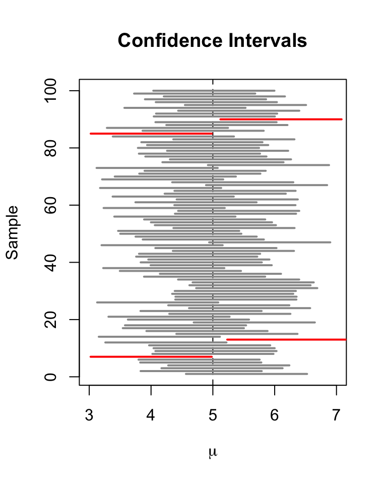
Interpreting confidence intervals

Capturing a proportion

• The confidence interval may or may not contain the true population proportion.

• Consider repeating the study over an over again, each time with the same sample size.

• Each time we would get a different $\hat{p}$

• From each $\hat{p}$, a different confidence interval could be computed.

• About 95% of these confidence intervals will capture the true proportion.

• 5% will be duds.

Random matters - confidence intervals

• There are a huge number of confidence intervals that could be drawn.

• In theory, all the confidence intervals could be listed.

  • 95% will “work” (capture the true proportion).
  • 5% will be “duds” (not capture the true proportion).

• What about our confidence interval (0.696, 1.044)?

  • In this case, we can find out the true value
  • Most of the time we never know

Random matters - confidence intervals

100 samples CI

Margin of error: certainty vs. precision

Margin of error

• Confidence interval for a population proportion: $\hat{p} \pm 2\times SE(\hat{p})$

• The distance, $~2\times SE(\hat{p})$, from $\hat{p}$ is called the margin of error

• Confidence intervals can be applied to many statistics, not just means. Regression slopes and other quantities can also have confidence intervals.

  • In general, a confidence interval has the form estimate $\pm$ margin of error

Certainty vs. precision

• Competing goals
  • More certainty, need to capture $p$ more often, need to make the interval wider.
  • More precise, need to provider tighter bounds on our estimate for $p$, need to make the interval narrower
• Instead of a 95% confidence interval, any percent can be used.
  • Increasing the confidence (e.g. 99%) increases the margin of error.
    • Need to make our range wider to make sure we don’t ‘miss’
  • Decreasing the confidence (e.g. 90%) decreases the margin of error.
    • Need to make our range smaller so as to be more specific about our guess

What sample size?

• Can increase both certainty and precision by increasing sample size

• For 95%, $z^*$ = 1.96

• Values that make ME largest are $\hat{p}=0.5$

• If we want to ensure, say, a margin of error of $<3$

  • $ME = z\times \sqrt{\frac{\hat{p}(1-\hat{p})}{n}}$
  • $0.03 = 1.96\times \sqrt{\frac{(0.5)(0.5)}{n}}$

• Solving for $n$, gives $n\approx1067.1$

• We need to survey at least 1068 to ensure a ME less than 0.03 for the 95% confidence interval.

Thoughts on sample size and ME

• Obtaining a large sample size can be expensive and/or take a long time.

• For a pilot study, $ME = 10$ can be acceptable.

• For full studies, $ME < 5$ is better.

• Public opinion polls typically use $ME = 3$, $n = 1000$

• If $p$ is expected to be very small such as 0.005, then much smaller ME such as 0.1% is required.

  • Common in medical studies